As a particle-based variational inference method, SVGD Liu & Wang, 2016 evolves a set of particles sampled from an initial distribution to collectively match any arbitrarily complex target distribution , as long as it is possible compute the score of . However, SVGD does not provide an explicit expression for the density it induces: while we can generate samples, we do not know the value of the corresponding probability density at those sampled points. That is, if we evolve for steps according to the SVGD update rule, we would obtain with , but we wouldn’t know the value of for a given . This is problematic when we are interested in downstream tasks such as likelihood-based evaluation, uncertainty quantification, or entropy estimation, as these require access to the density itself rather than just samples.
Derivation of the SVGD-induced Density
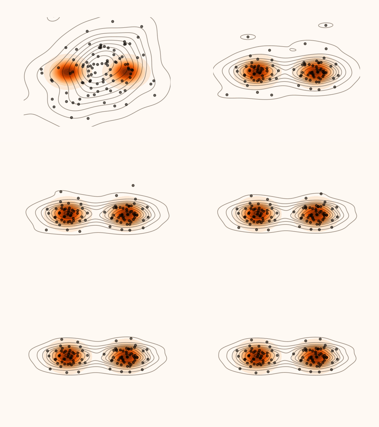
Figure 1:Density’ evolution starting from and following the SVGD velocity field.
Code for Figure 1.
from svgd.sampler import SVGD
from svgd.distributions import TorchDistribution
from svgd.kernels import RBF
from svgd.kernels.parameters import HeuristicKP
from svgd.lrs import ParameterLR
from svgd.callbacks import Logger

import torch
from torch.distributions import MixtureSameFamily, Categorical, Independent, Normal

import matplotlib
import pandas as pd
import seaborn as sns
import matplotlib.pyplot as plt
from matplotlib.animation import FuncAnimation

torch.manual_seed(0)

target_distribution = TorchDistribution(
    MixtureSameFamily(
        Categorical(torch.ones(2)),
        Independent(Normal(torch.tensor([[-1.0, 0.0], [1.0, 0.0]]), 1 / 3), 1),
    )
)
initial_distribution = TorchDistribution(Independent(Normal(torch.zeros(2), 1.0), 1))
kernel = RBF(HeuristicKP("median"))
lr = ParameterLR(torch.tensor(0.5))
logger = Logger(log_x=True)
logger.activated = True
svgd = SVGD(
    target_distribution=target_distribution,
    initial_distribution=initial_distribution,
    kernel=kernel,
    lr=lr,
    callbacks=[logger],
)

n_particles = 100
n_steps = 50
x, _, _ = svgd.sample(n_particles=n_particles, n_steps=n_steps)
x = x.detach()

bound = 2.5

grid = torch.arange(-bound, bound, 0.01)
xg, yg = torch.meshgrid(grid, grid, indexing="ij")
grid = torch.cat((xg.reshape(-1)[:, None], yg.reshape(-1)[:, None]), dim=-1)
zg = target_distribution.log_prob(grid).exp().view(xg.shape)

fig, ax = plt.subplots()
ax.pcolormesh(xg, yg, zg, cmap="Oranges")
ax.set_xlim(-bound, bound)
ax.set_ylim(-bound, bound)
ax.axis("off")
scatter = ax.scatter([], [], color="black", alpha=0.6)


def animate(frame):
    for artist in ax.collections:
        if isinstance(artist, matplotlib.contour.QuadContourSet):
            artist.remove()

    scatter.set_offsets(logger.x[frame])
    sns.kdeplot(
        x=logger.x[frame][:, 0],
        y=logger.x[frame][:, 1],
        ax=ax,
        alpha=0.4,
        color="black",
    )

    return (scatter,)


animation = FuncAnimation(
    fig,
    animate,
    len(logger.x),
    interval=1000 / 60,
    blit=False,
)
animation.save("density_evolution.gif", fps=120)
Suppose that, after SVGD steps, the particle is distributed according to . Then, using the change of variable formula for densities (CVF), the distribution of , where is the SVGD velocity field, is:
However, to apply the CVF, the SVGD transformation must be invertible. To ensure this, MET-SVGD adapts a sufficient conditions for the invertibility of transformations of the form from Behrmann et al. (2019) to SVGD. Namely, is invertible if , where denotes the spectral norm of .
In practice, it is easier to work with the log of the density, also called the log-likelihood:
Unfortunately, this expression involves the log of the determinant of a jacobian, which is expensive to compute. To avoid this, under the condition , MET-SVGD accurately estimates by , giving:
For samples , the trace term evaluated at is:
When is the RBF kernel, the first term in the above expression can be efficiently computed using only vector dot products. However, the second term is computationally expensive because it involves computing the trace of a hessian, which has complexity.
One way to altogether bypass computing this term is to estimate the expectation in using . However, this turns out to be suboptimal in the finite particle case. Instead, MET-SVGD efficiently estimates it as:
where satisfy and , and is the number of samples.
Since the estimator is weighted by , its variance is greatly reduced, and, in practice, only one is sufficient.
Unifying the Step-Size Conditions
The correctness of the previous derivation depends on two conditions:
to ensure that the SVGD transformation is invertible
for the approximation of to be accurate
While these are separate conditions, they can be unified by considering the order relation between the spectral norm of a real-valued square matrix and the magnitude of .
According to Wolkowicz & Styan (1980), for :
where and are the -th eigenvalue and singular value of , respectively.
Given that , we have:
Therefore, in order to satisfy both conditions, it is sufficient to choose the step-size such that:
Note that can be efficiently computed using only vector dot products and first-order derivatives, similarly to . And, in practice, MET-SVGD solves by taking the maximum over particles at iteration .
- Liu, Q., & Wang, D. (2016). Stein variational gradient descent: A general purpose bayesian inference algorithm. NeurIPS.
- Behrmann, J., Grathwohl, W., Chen, R. T., Duvenaud, D., & Jacobsen, J.-H. (2019). Invertible residual networks. ICML.
- Hutchinson, M. F. (1989). A stochastic estimator of the trace of the influence matrix for Laplacian smoothing splines. Commun. Stat. Simul. Comput.
- Song, Y., Garg, S., Shi, J., & Ermon, S. (2020). Sliced score matching: A scalable approach to density and score estimation. UAI.
- Wolkowicz, H., & Styan, G. P. (1980). Bounds for eigenvalues using traces. Linear Algebra Appl.