The SVGD Update Rule
Stein Variational Gradient Descent Liu & Wang, 2016 is a particle-based sampling algorithm that begins with samples drawn from an initial reference distribution and iteratively transports them via the SVGD velocity field . After enough iterations, the transformed particles form an empirical distribution that closely matches the target.
Formally, at iteration , the SVGD update rule is:
where is the -th particle at iteration , is the step-size, is the unnormalized density, and is a kernel function, most commonly the RBF kernel.
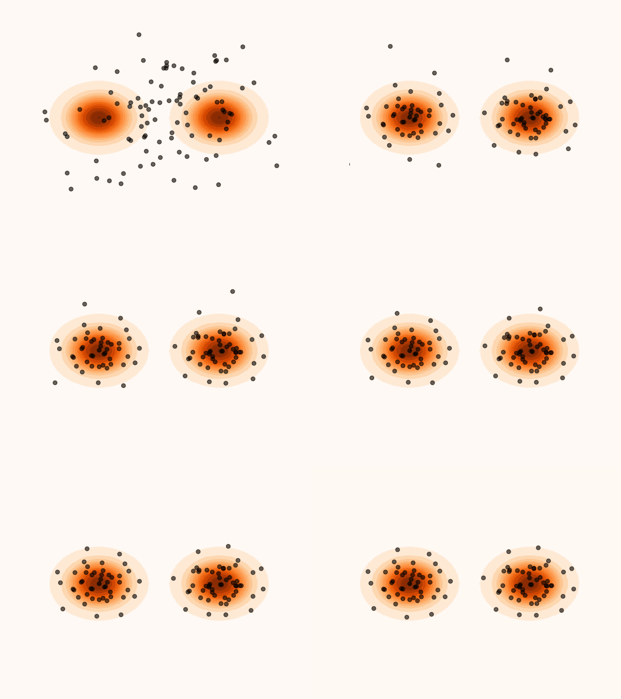
Figure 1:Particles’ evolution starting from and following the SVGD velocity field.
Code for Figure 1.
from svgd.sampler import SVGD
from svgd.distributions import TorchDistribution
from svgd.kernels import RBF
from svgd.kernels.parameters import HeuristicKP
from svgd.lrs import ParameterLR
from svgd.callbacks import Logger

import torch
from torch.distributions import MixtureSameFamily, Categorical, Independent, Normal

import matplotlib.pyplot as plt
from matplotlib.animation import FuncAnimation

torch.manual_seed(0)

target_distribution = TorchDistribution(
    MixtureSameFamily(
        Categorical(torch.ones(2)),
        Independent(Normal(torch.tensor([[-1.0, 0.0], [1.0, 0.0]]), 1 / 3), 1),
    )
)
initial_distribution = TorchDistribution(Independent(Normal(torch.zeros(2), 1.0), 1))
kernel = RBF(HeuristicKP("median"))
lr = ParameterLR(torch.tensor(0.5))
logger = Logger(log_x=True)
logger.activated = True
svgd = SVGD(
    target_distribution=target_distribution,
    initial_distribution=initial_distribution,
    kernel=kernel,
    lr=lr,
    callbacks=[logger],
)

n_particles = 100
n_steps = 50
x, _, _ = svgd.sample(n_particles=n_particles, n_steps=n_steps)
x = x.detach()

grid = torch.arange(-2, 2, 0.001)
xg, yg = torch.meshgrid(grid, grid, indexing="ij")
grid = torch.cat((xg.reshape(-1)[:, None], yg.reshape(-1)[:, None]), dim=-1)
zg = target_distribution.log_prob(grid).exp().view(xg.shape)

fig, ax = plt.subplots()
ax.pcolormesh(xg, yg, zg, cmap="Oranges")
ax.set_xlim(-2.0, 2.0)
ax.set_ylim(-2.0, 2.0)
ax.axis("off")
scatter = ax.scatter([], [], color="black", alpha=0.6)


def animate(frame):
    scatter.set_offsets(logger.x[frame])
    return (scatter,)


animation = FuncAnimation(
    fig,
    animate,
    len(logger.x),
    interval=1000 / 60,
    blit=False,
)
animation.save("particle_evolution.gif", fps=120)
A key property of SVGD is that the velocity field is chosen to maximally decrease the KL divergence between the particle distribution and the target. Intuitively, each update moves the particles in the direction that most closely makes their empirical distribution resemble the target distribution.
The RBF Kernel
The RBF kernel is defined as
where is the kernel bandwidth.
Using the RBF kernel, the SVGD update rule becomes:
In the drift term, the kernel value determines how strongly the particle is influenced by the score . This term moves particles toward regions of high probability. In the repulsion term, the same kernel value controls how far is pushed away from along the direction . This term enforces diversity among particles, preventing them from collapsing onto a single mode.
The kernel takes its maximum value of 1 when , and approaches 0 as . Intuitively, measures similarity between particles based on Euclidean distance, with the effective neighborhood size controlled by .
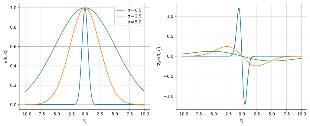
Figure 2:The neighborhood of as a function of in 1D in terms of similarity and repulsive force for different values.
Code for Figure 2.
import torch
import numpy as np
import pandas as pd
import seaborn as sns
import matplotlib.pyplot as plt

torch.manual_seed(0)

bound = 10.0
x = torch.arange(-bound, bound, 0.1).unsqueeze(-1)

sigma = torch.tensor([0.5, 2.5, 5.0])
gamma = sigma.pow(2).mul(2).pow(-1)

norm = x.pow(2).sum(-1)
k = gamma.unsqueeze(-1).mul(norm).mul(-1).exp()
k_xj = gamma.mul(2).unsqueeze(-1).unsqueeze(-1).mul(k.unsqueeze(-1)).mul(x.mul(-1))

data = pd.DataFrame(
    [
        {
            "sigma": s.item(),
            "x": x[idx, 0].item(),
            "k": k[s_idx, idx].item(),
            "k_xj": k_xj[s_idx, idx, 0].item(),
        }
        for s_idx, s in enumerate(sigma)
        for idx in range(x.shape[0])
    ]
)

r, c = 1, 2
fig, ax = plt.subplots(r, c, figsize=(6.4 * c, 4.8 * r))

if c == 1:
    ax = np.array([ax])

if r == 1:
    ax = np.array([ax])

sns.lineplot(
    data,
    x="x",
    y="k",
    hue="sigma",
    ax=ax[0, 0],
    palette=sns.color_palette("tab10"),
)
ax[0, 0].grid()
ax[0, 0].set_ylabel("$\\kappa(0, x_j^l)$")
ax[0, 0].set_xlabel("$x_j^l$")

sns.lineplot(
    data,
    x="x",
    y="k_xj",
    hue="sigma",
    ax=ax[0, 1],
    palette=sns.color_palette("tab10"),
)
ax[0, 1].grid()
ax[0, 1].set_ylabel("$\\nabla_{x_j^l} \\kappa(0, x_j^l)$")
ax[0, 1].set_xlabel("$x_j^l$")

handles, labels = ax[0, 0].get_legend_handles_labels()
labels = [f"$\\sigma = {label}$" for label in labels]

ax[0, 0].legend_.remove()
ax[0, 1].legend_.remove()

legend = fig.legend(
    handles,
    labels,
    loc="lower center",
    bbox_to_anchor=(0.42, 0.7),
    framealpha=1.0,
)

fig.savefig("bandwidth.svg", bbox_inches="tight")
Choosing an appropriate value for is nontrivial: both extremely small and extremely large bandwidths cause the repulsion term to vanish. A common heuristic is the median trick, which sets , where is the number of particles. This choice roughly ensures that .
However, it is not obvious that this property is always desirable, and in practice the median trick can be somewhat brittle depending on the geometry of the target distribution.
Derivation of the SVGD Update Rule
Suppose we want to sample from a target distribution . Given , the idea behind SVGD is to find a velocity field that maximally decreases the KL divergence between the distribution of and , which we denote as . Note that , since .
For a small enough , we can approximate with its taylor expansion with respect to around 0:
We can, therefore, estimate the decrease in the KL divergence as:
Hence, since and are independent, finding that maximizes this decrease is approximately equivalent to finding that maximizes . This becomes exact as , in which case we are looking for that maximizes the instantaneous decrease in .
Formally, we want to solve the following optimization problem:
where is a suitable family of functions.
Let . One can show that , where is the distribution of , assuming that is invertible. This allows us to get a closed form expression of the gradient of with respect to , as is independent of :
In case is a subset of , where is a Reproducing Kernel Hilbert Space (RKHS) with a corresponding kernel , then, using the reproducing property of the RKHS, can be written as . Given this, we can rewrite the gradient of the KL divergence as an inner product:
If we constrain the norm of in , so that , the maximum of the inner product is achieved when is proportional to the second argument, hence the maximizer is:
For a distribution known up to a normalization constant , , which does not depend on the normalization constant .
- Liu, Q., & Wang, D. (2016). Stein variational gradient descent: A general purpose bayesian inference algorithm. NeurIPS.