Energy-Based Models
Energy-based models (EBMs) are generative models that learn a density parametrized by an energy function , so that , with . Typically, EBMs are trained via maximum likelihood estimation (MLE) by estimating the gradient of the maximum likelihood loss, since direct computation of the loss is not feasible due to the intractability of . However, when a sampler with a tractable density is given, a tight lower bound on the MLE loss can be computed:
The EBM is then trained by alternating between maximizing with respect to to further tighten the lower bound, and minimizing it with respect to .
In Figure 1, we show the Fréchet Inception Distance (FID) averaged over 5 random seeds for CIFAR10 image generation. We compare against P-SVGD Messaoud et al., 2024 and Glow (Normalizing Flow) Kingma & Dhariwal, 2018.
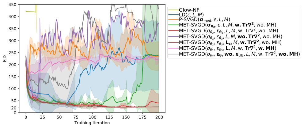
Figure 1:FID on CIFAR-10; bold marks changes between configurations.
Removing either the trace-of-Hessian term or the step-size bound causes the training to diverge, as the violet and gray curves show. Figure 2 shows that adding the trace-of-Hessian term produces smoother energy landscapes that are much easier to sample from. The step-size bound plays a different but equally important role, as it ensures that the entropy estimation remains valid.
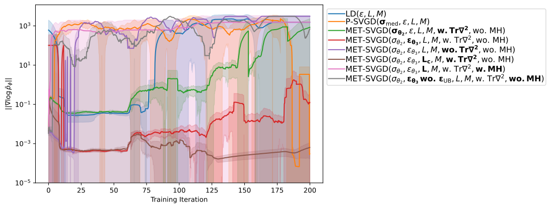
Figure 2:Smoothness of the learnt EBM as measured by throughout training iterations. The configurations with the best FID (Figure 1) exhibit smoother landscapes.
Replacing the median heuristic bandwidth, , with a learnable bandwidth greatly improves stability and leads to significantly better FID scores compared to P-SVGD (green versus orange). As shown in Figure 3a, the median heuristic bandwidth is on average more than an order of magnitude larger than the learned value . This overly large bandwidth causes particles to become spuriously correlated, hurting sample quality.
Learning the step size as well (red curve) allows the method to converge to the target distribution much faster. Figure 3b illustrates that the learned step size is much larger than the fixed step size .

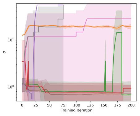
(a)Kernel bandwidth across training iterations.
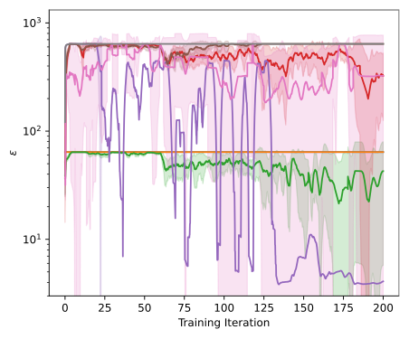
(b)Step-size across training iterations
Figure 3:Learnt kernel bandwidth and step-size across training iterations. The trends exhibited by the learnt kernel bandwidth and step-size in MET-SVGD configurations are significantly different from and constant .
Using an adaptive number of update steps further stabilizes training, as shown by the brown curve.
In contrast to the other MET-SVGD optimizations, experiments that incorporate MH diverge, as indicated by the pink curve. This instability is not inherent to MET-SVGD itself, but instead comes from the interaction between MH rejection dynamics and a the loss function, , not being lower-bounded. The stability of the training objective depends critically on the quality of the samples used to estimate the expectation with respect to the sampler. When the energy landscape is highly complex, MH acceptance rates can become very low Figure 4, preventing particles from moving toward high-density regions of the target distribution. As a result, sample quality degrades and training eventually diverges.
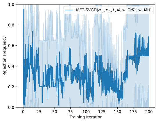
Figure 4:MH rejection rate across training iterations.
Glow-NF exhibits a similar failure mode, struggling to produce good samples early in training and ultimately diverging as well.
Maximum Entropy Reinforcement Learning
MaxEnt RL learns a stochastic policy over actions given a state by maximizing the sum of expected rewards and entropies:
We model the sampler and estimate the entropy using the MET-SVGD framework and compare against SAC Haarnoja et al., 2018, which models the policy as a diagonal Gaussian, SAC-NF, which models the policy as an auto-regressive normalizing flow Papamakarios et al., 2017, and P-SVGD Messaoud et al., 2024. In Figure 5, we report the average return on 10 rollouts every 1000 steps on Walker2d-v2 averaged over 5 seeds.

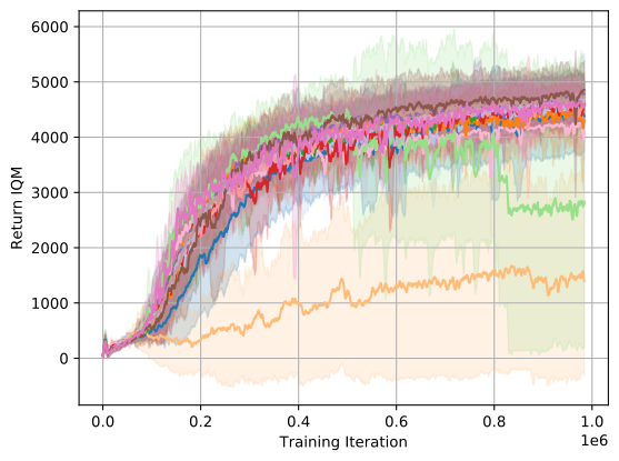
(a)Return IQM across training iterations.
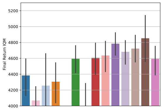
(b)Return IQM at the end of training.
Figure 5:Return IQM on Walker2d-v2.
Learning the kernel bandwidth (orange) and adding the trace-of-Hessian correction (green) both lead to substantial improvements over the P-SVGD baseline. In contrast, removing the bound on the step size (pale green) causes the method to diverge, which is expected.
Learning the step size without the trace-of-Hessian term (peach) performs worse than all baselines. In this case, particles tend to drift into non-smooth regions of the landscape Figure 6.
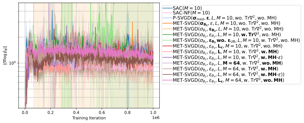
Figure 6:Smoothness as measured by throughout training iterations.
The best results come from incorporating MH with an -greedy schedule (purple): applying MH with high probability later in training and low probability early on helps balance exploration in the beginning with exploitation as learning progresses. These improvements become even more pronounced when we increase the number of particles from 10 to 64 (brown).
- Messaoud, S., Mokeddem, B., Xue, Z., Pang, L., An, B., Chen, H., & Chawla, S. (2024). S 2 AC: Energy-Based Reinforcement Learning with Stein Soft Actor Critic. ICLR.
- Kingma, D. P., & Dhariwal, P. (2018). Glow: Generative flow with invertible 1x1 convolutions. NeurIPS.
- Haarnoja, T., Zhou, A., Abbeel, P., & Levine, S. (2018). Soft actor-critic: Off-policy maximum entropy deep reinforcement learning with a stochastic actor. ICML.
- Papamakarios, G., Pavlakou, T., & Murray, I. (2017). Masked autoregressive flow for density estimation. NeurIPS.