
Figure 1:Overview of the MET-SVGD framework.
End-to-End SVGD Parameter Learning via Reverse KL Minimization
Although we consistently observe the particle converging to the high density regions of the target distributions for different values of the kernel bandwidth , using the derived closed-form expression of the SVGD-induced density to estimate the entropy of the target is very sensitive to the choice of , in the sense that the estimate only converges to the true entropy for specific values.
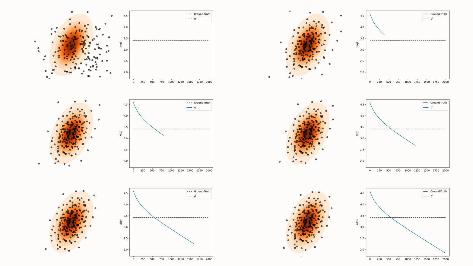
(a)Particle and entropy evolution with .
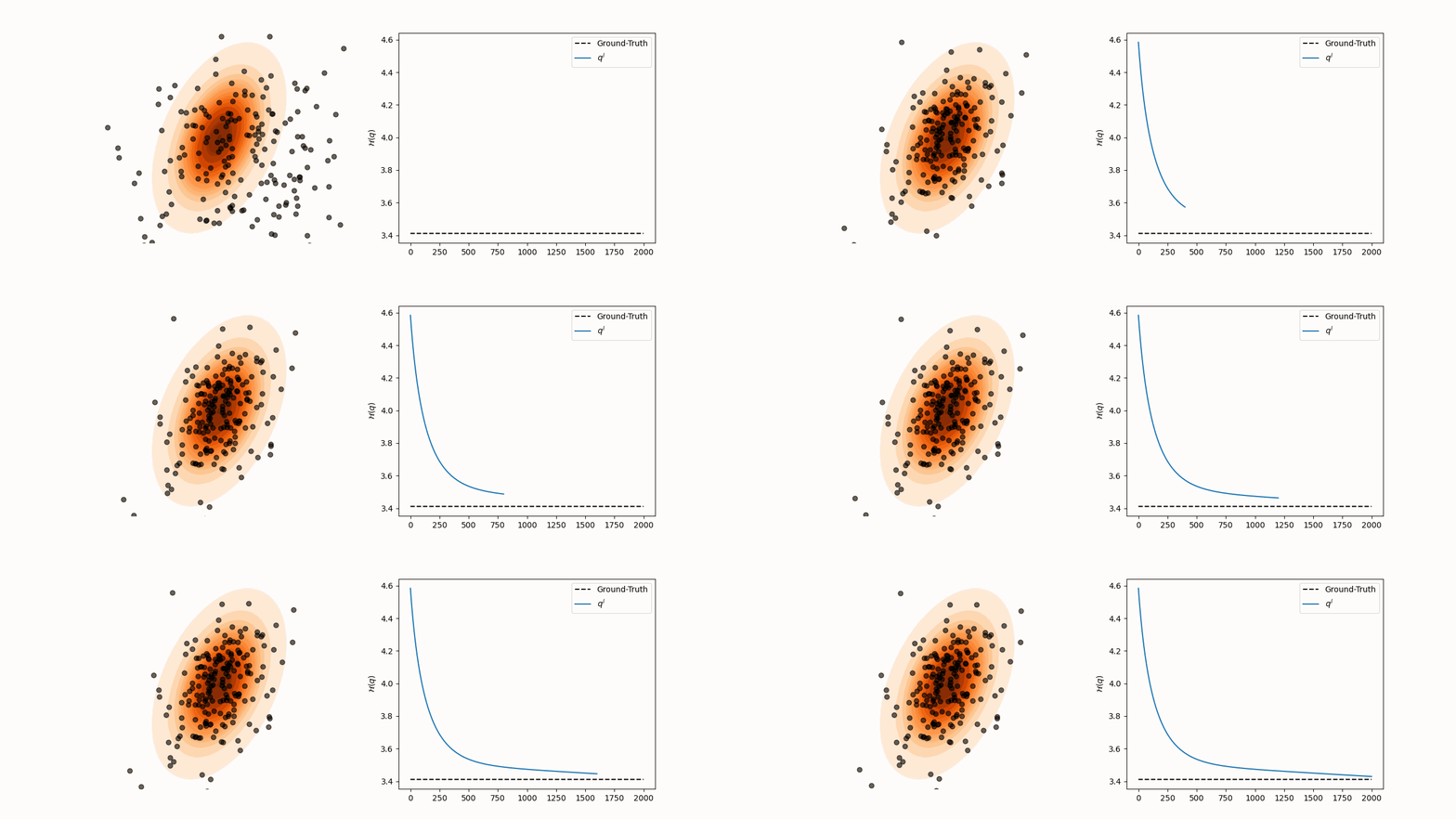
(b)Particle and entropy evolution with .
Figure 2:Particle and entropy evolution for different values. The convergence of the entropy estimate to the true value depends on the choice of despite particles’ convergence to the target.
Code for Figure 2.
from svgd.sampler import SVGD
from svgd.distributions import TorchDistribution, Gaussian
from svgd.kernels import RBF
from svgd.kernels.parameters import HeuristicKP, ParameterKP
from svgd.lrs import ParameterLR
from svgd.callbacks import Logger

import torch
from torch.distributions import MultivariateNormal

import matplotlib.pyplot as plt
from matplotlib.animation import FuncAnimation

torch.manual_seed(0)

sigma_choice = "1"

mu_x, mu_y = -0.6871, 0.8010
target_distribution = TorchDistribution(
    MultivariateNormal(
        torch.Tensor([mu_x, mu_y]),
        torch.Tensor([[0.2260, 0.1652], [0.1652, 0.6779]]).mul(5),
    )
)
initial_distribution = Gaussian(torch.zeros(2), torch.ones(2).mul(6).sqrt())
sigma = (
    HeuristicKP("median")
    if sigma_choice == "median"
    else ParameterKP(torch.tensor(float(sigma_choice)))
)
kernel = RBF(sigma)
lr = ParameterLR(torch.tensor(0.1))
logger = Logger(log_x=True, log_log_q=True)
logger.activated = True
svgd = SVGD(
    target_distribution=target_distribution,
    initial_distribution=initial_distribution,
    kernel=kernel,
    lr=lr,
    callbacks=[logger],
)

n_particles = 200
n_steps = 2000
x, _, _ = svgd.sample_with_log_q(n_particles=n_particles, n_steps=n_steps)
x = x.detach()

bound = 5
grid_x = torch.arange(mu_x - bound, mu_x + bound, 0.01)
grid_y = torch.arange(mu_y - bound, mu_y + bound, 0.01)
xg, yg = torch.meshgrid(grid_x, grid_y, indexing="ij")
grid = torch.cat((xg.reshape(-1)[:, None], yg.reshape(-1)[:, None]), dim=-1)
zg = target_distribution.log_prob(grid).exp().view(xg.shape)

fig, ax = plt.subplots(1, 2, figsize=(6.4 * 2, 4.8))

ax[0].pcolormesh(xg, yg, zg, cmap="Oranges")
ax[0].set_xlim(mu_x - bound, mu_x + bound)
ax[0].set_ylim(mu_y - bound, mu_y + bound)
ax[0].set_axis_off()
scatter = ax[0].scatter([], [], color="black", alpha=0.6)
scatter = ax[0].scatter(*x.T, color="black", alpha=0.6)

ax[1].plot(
    [target_distribution.distribution.entropy() for _ in range(n_steps)],
    color="black",
    ls="--",
    label="Ground-Truth",
)
plot = ax[1].plot([-log_q for log_q in logger.log_q], label="$q^l$")[0]
plot.set_xdata([])
plot.set_ydata([])
ax[1].set_ylabel("$\\mathcal{H}(q)$")
ax[1].legend()

x_data = list(range(len(logger.x)))
y_data = [-log_q for log_q in logger.log_q]


def animate(frame):
    scatter.set_offsets(logger.x[min(frame, len(logger.x) - 1)])
    plot.set_xdata(x_data[:frame])
    plot.set_ydata(y_data[:frame])
    return (scatter, plot)


animation = FuncAnimation(
    fig,
    animate,
    list(range(0, n_steps + 20, 20)),
    interval=1000 / 60,
    blit=False,
)
animation.save(f"sensitivity_{sigma_choice}.gif", fps=120)
The target’s entropy estimate based on is:
As , we expect and the trace term above to converge zero in expectation. However, this is not trivial from the perspective of selection. It can be shown via a taylor expansion that this trace term corresponds to an 8-th degree polynomial in , with coefficients that do not guarantee the existence of real roots.
To resolve this, MET-SVGD transforms the hyperparameter selection problem into a parameter learning one by leveraging the computed to minimize the KL divergence between and , thus obtaining both the optimal kernel bandwidth and step-size for every step :
where is the step-size upper bound derived in Section 3.2.
Learning the step-size alongside the kernel bandwidth is necessary, since, from the argument above, the kernel bandwidth alone might not be enough for the trace term to converge to zero.
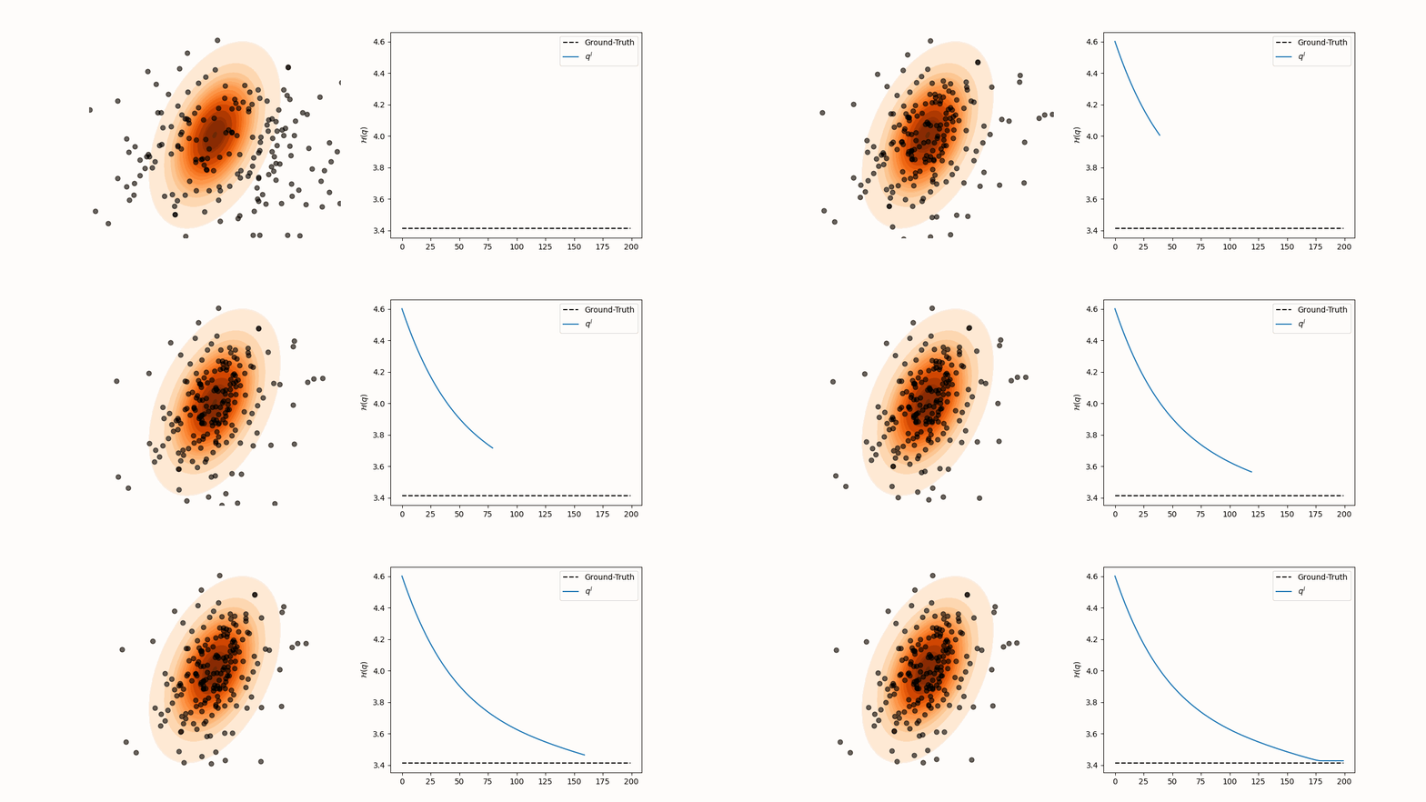
Figure 3:Particle and entropy evolution with learnable kernel bandwidth and step-size.
Code for Figure 3.
from svgd.sampler import SVGD
from svgd.distributions import TorchDistribution, Gaussian
from svgd.kernels import RBF
from svgd.kernels.parameters import StepParameterKP
from svgd.lrs import StepLR
from svgd.callbacks import Logger

import torch
from torch.optim.adam import Adam
from torch.distributions import MultivariateNormal

from tqdm import tqdm
import matplotlib.pyplot as plt
from matplotlib.animation import FuncAnimation

torch.manual_seed(0)

device = "cuda:0"
n_epochs = 100
n_particles = 200
n_steps = 200

mu_x, mu_y = -0.6871, 0.8010
target_distribution = TorchDistribution(
    MultivariateNormal(
        torch.Tensor([mu_x, mu_y]).to(device),
        torch.Tensor([[0.2260, 0.1652], [0.1652, 0.6779]]).mul(5).to(device),
    )
)
initial_distribution = Gaussian(
    torch.zeros(2), torch.ones(2).mul(6).sqrt()
).requires_grad_(False)
sigma = StepParameterKP(torch.zeros(n_steps), lambda x: x.exp())
kernel = RBF(sigma)
lr = StepLR(torch.tensor(0.1), torch.tensor(n_steps - 20), torch.tensor(1e-6))
lr._log_step_size.requires_grad_(False)
lr._log_decay_rate.requires_grad_(False)
logger = Logger(log_x=True, log_log_q=True)
svgd = SVGD(
    target_distribution=target_distribution,
    initial_distribution=initial_distribution,
    kernel=kernel,
    lr=lr,
    bound_lr=True,
    ij_term_density=True,
    callbacks=[logger],
).to(device)
optimizer = Adam(svgd.parameters(), 1e-2)

for epoch in tqdm(range(n_epochs)):
    logger.activated = epoch == n_epochs - 1
    x, _, log_q = svgd.sample_with_log_q(n_particles=n_particles, n_steps=n_steps)
    log_q = log_q.mean()
    log_p = target_distribution.log_prob(x).mean()
    kld = log_q.sub(log_p)
    kld.backward()
    optimizer.step()
    optimizer.zero_grad()

bound = 5
grid_x = torch.arange(mu_x - bound, mu_x + bound, 0.01)
grid_y = torch.arange(mu_y - bound, mu_y + bound, 0.01)
xg, yg = torch.meshgrid(grid_x, grid_y, indexing="ij")
grid = torch.cat((xg.reshape(-1)[:, None], yg.reshape(-1)[:, None]), dim=-1)
zg = target_distribution.log_prob(grid.to(device)).exp().view(xg.shape).cpu()

fig, ax = plt.subplots(1, 2, figsize=(6.4 * 2, 4.8))

ax[0].pcolormesh(xg, yg, zg, cmap="Oranges")
ax[0].set_xlim(mu_x - bound, mu_x + bound)
ax[0].set_ylim(mu_y - bound, mu_y + bound)
ax[0].set_axis_off()
scatter = ax[0].scatter([], [], color="black", alpha=0.6)
scatter = ax[0].scatter(*x.detach().cpu().T, color="black", alpha=0.6)

ax[1].plot(
    [target_distribution.distribution.entropy().item() for _ in range(n_steps)],
    color="black",
    ls="--",
    label="Ground-Truth",
)
plot = ax[1].plot([-log_q for log_q in logger.log_q], label="$q^l$")[0]
plot.set_xdata([])
plot.set_ydata([])
ax[1].set_ylabel("$\\mathcal{H}(q)$")
ax[1].legend()

x_data = list(range(len(logger.x)))
y_data = [-log_q for log_q in logger.log_q]


def animate(frame):
    scatter.set_offsets(logger.x[min(frame, len(logger.x) - 1)])
    plot.set_xdata(x_data[:frame])
    plot.set_ydata(y_data[:frame])
    return (scatter, plot)


animation = FuncAnimation(
    fig,
    animate,
    list(range(0, n_steps + 2, 2)),
    interval=1000 / 60,
    blit=False,
)
animation.save(f"sensitivity_metsvgd.gif", fps=120)
Faster Convergence via Learning the Initial Distribution
To accelerate convergence, MET-SVGD also learns the initial distribution . This is done via reverse KL minimization, similar to learning the kernel bandwidth and step-size.
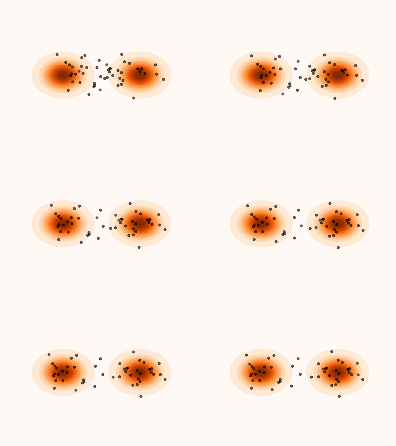
(a)Particle’s evolution with a learned initial distribution.
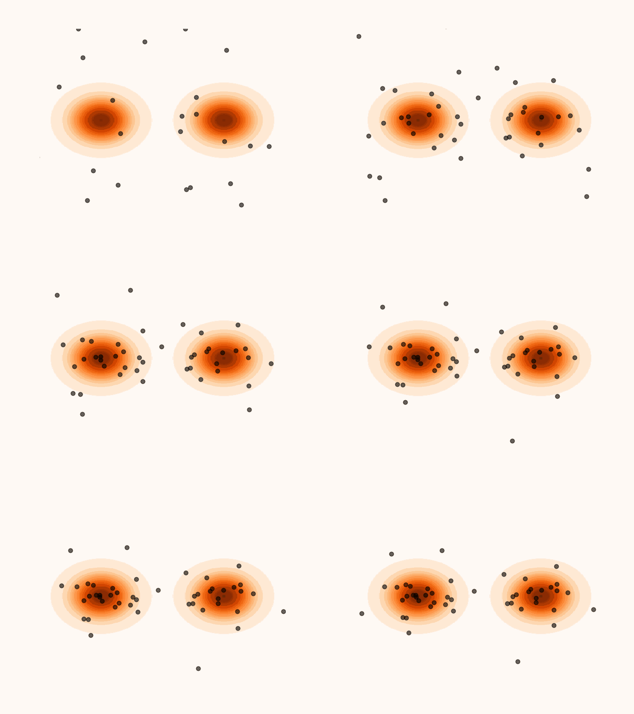
(b)Particle’s evolution with a pre-specified initial distribution.
Figure 4:Learning the initial distribution leads to faster convergence.
Code for Figure 4.
from svgd.sampler import SVGD
from svgd.distributions import TorchDistribution, Gaussian
from svgd.kernels import RBF
from svgd.kernels.parameters import ParameterKP
from svgd.lrs import StepLR
from svgd.callbacks import Logger

import torch
from torch.optim.adam import Adam
from torch.distributions import MixtureSameFamily, Categorical, Independent, Normal

from tqdm import tqdm
import matplotlib.pyplot as plt
from matplotlib.animation import FuncAnimation

from copy import deepcopy

torch.manual_seed(0)

device = "cuda:0"

n_epochs = 300
n_particles = 50
n_steps = 100

target_distribution = TorchDistribution(
    MixtureSameFamily(
        Categorical(torch.ones(2).to(device)),
        Independent(
            Normal(torch.tensor([[-1.0, 0.0], [1.0, 0.0]]).to(device), 1 / 3), 1
        ),
    )
)
initial_distribution = Gaussian(torch.zeros(2), torch.ones(2).mul(2.0)).to(device)
initial_distribution.mu.requires_grad_(False)
sigma = ParameterKP(torch.tensor(0.0), lambda x: x.exp()).to(device)
kernel = RBF(sigma)
lr = StepLR(
    torch.tensor(0.1),
    torch.tensor(n_steps / 2),
    torch.tensor(1e-9),
).to(device)
lr._log_decay_rate.requires_grad_(False)
lr._log_initial_lr.requires_grad_(False)
logger = Logger(log_x=True)
logger.activated = True
svgd = SVGD(
    target_distribution=target_distribution,
    initial_distribution=initial_distribution,
    kernel=kernel,
    lr=lr,
    bound_lr=True,
    ij_term_density=True,
    leaky_lr_clamp=True,
    callbacks=[logger],
).to(device)
svgd_fixed = deepcopy(svgd)
svgd_fixed.initial_distribution.requires_grad_(False)
logger_fixed: Logger = svgd_fixed.callbacks[0]
optimizer = Adam(svgd.parameters(), 1e-2)
optimizer_fixed = Adam(svgd_fixed.parameters(), 1e-2)


def optimize_svgd(svgd: SVGD, n_steps: int, optimizer: Adam):
    x, _, log_q = svgd.sample_with_log_q(n_particles=n_particles, n_steps=n_steps)
    log_q = log_q.mean()
    log_p = target_distribution.log_prob(x).mean()
    kld = log_q.sub(log_p)
    kld.backward()
    optimizer.step()
    optimizer.zero_grad()


for epoch in tqdm(range(n_epochs)):
    optimize_svgd(svgd, n_steps, optimizer)
    optimize_svgd(svgd_fixed, n_steps, optimizer_fixed)

grid = torch.arange(-2, 2, 0.01)
xg, yg = torch.meshgrid(grid, grid, indexing="ij")
grid = torch.cat((xg.reshape(-1)[:, None], yg.reshape(-1)[:, None]), dim=-1)
zg = target_distribution.log_prob(grid.to(device)).exp().view(xg.shape).cpu()

fig, ax = plt.subplots(1, 1, figsize=(6.4 * 1, 4.8 * 1))
ax.pcolormesh(xg, yg, zg, cmap="Oranges")
ax.set_xlim(-2.0, 2.0)
ax.set_ylim(-2.0, 2.0)
ax.axis("off")
scatter = ax.scatter([], [], color="black", alpha=0.6)


def animate(frame, logger):
    scatter.set_offsets(logger.x[frame])
    return (scatter,)


FuncAnimation(
    fig,
    lambda frame: animate(frame, logger),
    range(len(logger.x)),
    interval=1000 / 60,
    blit=False,
).save("particle_evolution_learnable_1.gif", fps=120)
FuncAnimation(
    fig,
    lambda frame: animate(frame, logger_fixed),
    range(len(logger.x)),
    interval=1000 / 60,
    blit=False,
).save("particle_evolution_learnable_2.gif", fps=120)
Stein-Identity as a Stopping Criterion
In SVGD, the number of steps for which the algorithm is run is specified is a hyperparameter that must be tuned for each target distribution . This is also typically the case for some MCMC algorithms such as Langevin Dynamics. MET-SVGD on the other hand employs an adaptive number of steps by checking at each step whether convergence has been achieved by measuring the violation of Stein’s Identity:
which only incurs a vector dot product to compute, as and have already been computed.
Based on this, MET-SVGD can be viewed as a normalizing flow model with a full-rank Jacobian and an adaptive number of layers, retaining computational efficiency without sacrificing expressivity.
Divergence Control via Metropolis-Hastings
In many application, the unnormalized density may exhibit abrupt gradient changes or contain highly non-smoothness regions, which can lead to instability or divergence during sampling.
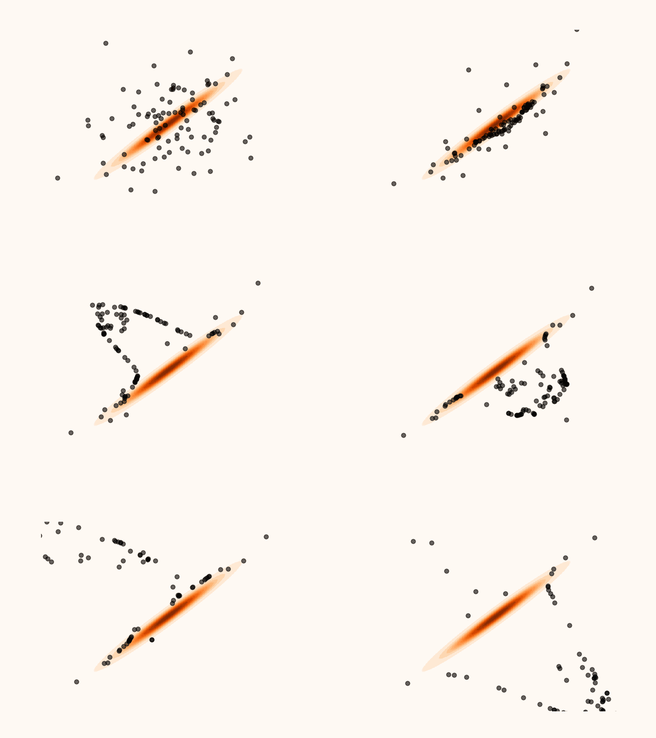
Figure 5:Particles’ evolution in the presence of non-smoothness.
Code for Figure 5.
from svgd.sampler import SVGD
from svgd.distributions import TorchDistribution
from svgd.kernels import RBF
from svgd.kernels.parameters import HeuristicKP
from svgd.lrs import ParameterLR
from svgd.callbacks import Logger

import torch
from torch.distributions import MultivariateNormal, Independent, Normal

import matplotlib.pyplot as plt
from matplotlib.animation import FuncAnimation

torch.manual_seed(0)

phi = torch.tensor(torch.pi / 4)
cos = torch.cos(phi)
sin = torch.sin(phi)
rotation = torch.tensor([[cos, -sin], [sin, cos]])
cov = torch.tensor([[1.0, 0.0], [0.0, 1e-2]])
cov = rotation @ cov @ rotation.T
target_distribution = TorchDistribution(MultivariateNormal(torch.zeros(2), cov))
initial_distribution = TorchDistribution(Independent(Normal(torch.zeros(2), 1.0), 1))
kernel = RBF(HeuristicKP("median"))
lr = ParameterLR(torch.tensor(0.1))
logger = Logger(log_x=True)
logger.activated = True
svgd = SVGD(
    target_distribution=target_distribution,
    initial_distribution=initial_distribution,
    kernel=kernel,
    lr=lr,
    callbacks=[logger],
)

n_particles = 100
n_steps = 25
x, _, _ = svgd.sample(n_particles=n_particles, n_steps=n_steps)
x = x.detach()

bound = 3.0

grid = torch.arange(-bound, bound, 0.01)
xg, yg = torch.meshgrid(grid, grid, indexing="ij")
grid = torch.cat((xg.reshape(-1)[:, None], yg.reshape(-1)[:, None]), dim=-1)
zg = target_distribution.log_prob(grid).exp().view(xg.shape)

fig, ax = plt.subplots()
ax.pcolormesh(xg, yg, zg, cmap="Oranges")
ax.set_xlim(-bound, bound)
ax.set_ylim(-bound, bound)
ax.axis("off")
scatter = ax.scatter([], [], color="black", alpha=0.6)


def animate(frame):
    scatter.set_offsets(logger.x[frame])
    return (scatter,)


animation = FuncAnimation(
    fig,
    animate,
    len(logger.x),
    interval=1000 / 60,
    blit=False,
)
animation.save("particle_evolution_non_smooth.gif", fps=120)
MET-SVGD addresses this issue by introducing a principled divergence control mechanism based on Metropolis-Hastings Tierney, 1994. At each step , the SVGD update is interpreted as a proposal distribution, yielding a proposed state . This proposal is accepted with probability , in which case . Otherwise, the proposal is rejected and the previous state is retained, i.e. .
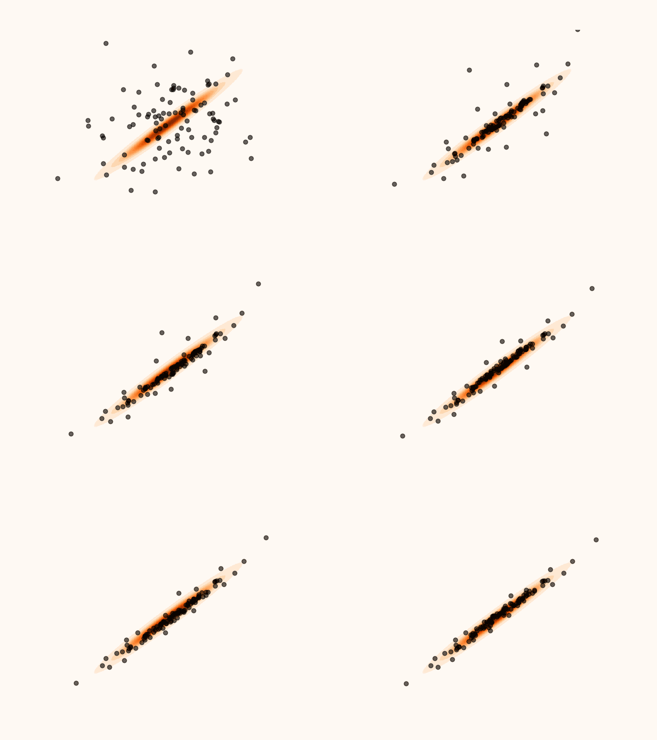
Figure 6:Particles’ evolution in the presence of non-smoothness with MH divergence control.
Code for Figure 6.
from svgd.sampler import SVGD
from svgd.distributions import TorchDistribution
from svgd.kernels import RBF
from svgd.kernels.parameters import HeuristicKP
from svgd.lrs import ParameterLR
from svgd.callbacks import Logger

import torch
from torch.distributions import MultivariateNormal, Independent, Normal

import matplotlib.pyplot as plt
from matplotlib.animation import FuncAnimation

torch.manual_seed(0)

phi = torch.tensor(torch.pi / 4)
cos = torch.cos(phi)
sin = torch.sin(phi)
rotation = torch.tensor([[cos, -sin], [sin, cos]])
cov = torch.tensor([[1.0, 0.0], [0.0, 1e-2]])
cov = rotation @ cov @ rotation.T
target_distribution = TorchDistribution(MultivariateNormal(torch.zeros(2), cov))
initial_distribution = TorchDistribution(Independent(Normal(torch.zeros(2), 1.0), 1))
kernel = RBF(HeuristicKP("median"))
lr = ParameterLR(torch.tensor(0.1))
logger = Logger(log_x=True)
logger.activated = True
svgd = SVGD(
    target_distribution=target_distribution,
    initial_distribution=initial_distribution,
    kernel=kernel,
    lr=lr,
    divergence_control="metropolis-hastings",
    callbacks=[logger],
)

n_particles = 100
n_steps = 25
x, _, _ = svgd.sample(n_particles=n_particles, n_steps=n_steps)
x = x.detach()

bound = 3.0

grid = torch.arange(-bound, bound, 0.01)
xg, yg = torch.meshgrid(grid, grid, indexing="ij")
grid = torch.cat((xg.reshape(-1)[:, None], yg.reshape(-1)[:, None]), dim=-1)
zg = target_distribution.log_prob(grid).exp().view(xg.shape)

fig, ax = plt.subplots()
ax.pcolormesh(xg, yg, zg, cmap="Oranges")
ax.set_xlim(-bound, bound)
ax.set_ylim(-bound, bound)
ax.axis("off")
scatter = ax.scatter([], [], color="black", alpha=0.6)


def animate(frame):
    scatter.set_offsets(logger.x[frame])
    return (scatter,)


animation = FuncAnimation(
    fig,
    animate,
    len(logger.x),
    interval=1000 / 60,
    blit=False,
)
animation.save("particle_evolution_non_smooth_mh.gif", fps=120)
To inherit the convergence guarantees of Metropolis–Hastings (MH), MET-SVGD augments the SVGD state with a simple auxiliary random variable that can take one of two values, or 1. At each step , is sampled at random and determines how the proposal is constructed. If the value is 1, the SVGD transformation is applied in the usual forward direction; if it is , the inverse SVGD transformation is applied. This construction allows MET-SVGD to inherit MH convergence guarantees while still leveraging the efficiency of SVGD.
When is a Rademacher random variable, the probability of acceptance is computed as:
With the inclusion of the MH correction, the induced distribution given becomes:
and is obtained via marginalization, with .
Given that MET-SVGD inherits the convergence guarantees of MH, converges to the target distribution as , independently of the number of particles . By contrast, existing convergence guarantees for SVGD in the literature require both Sun et al., 2023.
- Tierney, L. (1994). Markov Chains for Exploring Posterior Distributions. The Annals of Statistics.
- Sun, L., Karagulyan, A., & Richtarik, P. (2023). Convergence of Stein variational gradient descent under a weaker smoothness condition. AISTATS.